Secant Method

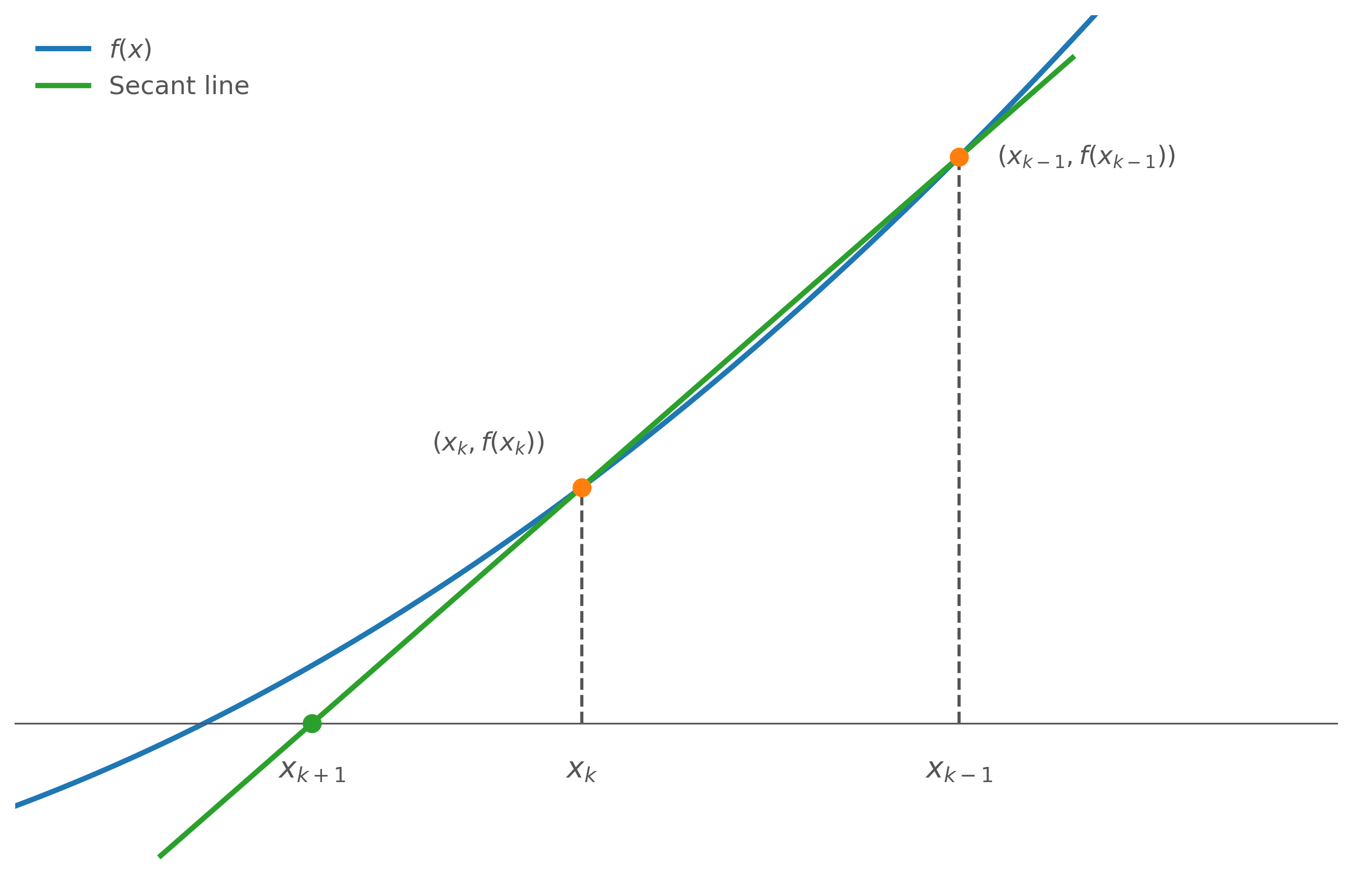
Newton’s method requires the analytical derivative $f'(x_k)$ at every step. When the function is too complicated to differentiate, or when only function values (not derivatives) are available, the secant method provides a practical alternative. It replaces the exact derivative with a finite difference approximation constructed from the two most recent iterates.

---

Motivation

Recall from numerical differentiation that the backward difference formula approximates the derivative:

$f'(x_k) \approx \frac{f(x_k) - f(x_{k-1})}{x_k - x_{k-1}}$

Substituting this approximation directly into Newton’s formula:

$x_{k+1} = x_k - \frac{f(x_k)}{f'(x_k)} \approx x_k - \frac{f(x_k)}{\dfrac{f(x_k) - f(x_{k-1})}{x_k - x_{k-1}}}$

Simplifying gives the secant method formula.

---

Formula

$\boxed{x_{k+1} = x_k - \frac{f(x_k)\,(x_k - x_{k-1})}{f(x_k) - f(x_{k-1})}}$

Unlike Newton’s method, which requires only one starting point $x_0$, the secant method requires two starting points $x_0$ and $x_1$ to compute the very first iterate $x_2$.

Note

Geometric Intuition: The secant method draws a straight secant line through the two most recent points on the curve: $(x_{k-1},\, f(x_{k-1}))$ and $(x_k,\, f(x_k))$. It defines the next point, $x_{k+1}$, as the exact x-intercept of that line. This is geometrically analogous to Newton’s method, but it bypasses the need for a tangent (derivative) by using two previous function evaluations instead.

---

Comparison with Newton’s Method

Property	Newton’s Method	Secant Method
Derivative required	Yes, $f'(x_k)$ at each step	No
Starting points needed	1 (just $x_0$)	2 ($x_0$ and $x_1$)
Convergence rate	Super-linear ($\lambda = 0$)	Super-linear (order $\approx 1.618$)
Cost per iteration	1 function + 1 derivative evaluation	1 function evaluation (derivative is reused)

The secant method converges slightly slower than Newton’s method in theory, but avoids the need for any derivative, making it the preferred choice when differentiation is expensive or impossible.

---

Worked Example

Problem: Find the root of $f(x) = \dfrac{1}{x} - 0.5$ using the secant method with $x_0 = 0.25$ and $x_1 = 0.5$.

Step 1 — Evaluate at the starting points

$f(x_0) = f(0.25) = \frac{1}{0.25} - 0.5 = 4 - 0.5 = 3.5$

$f(x_1) = f(0.5) = \frac{1}{0.5} - 0.5 = 2 - 0.5 = 1.5$

Step 2 — Compute $x_2$

$x_2 = x_1 - \frac{f(x_1)(x_1 - x_0)}{f(x_1) - f(x_0)} = 0.5 - \frac{1.5\,(0.5 - 0.25)}{1.5 - 3.5}$

$= 0.5 - \frac{1.5 \times 0.25}{-2} = 0.5 - \frac{0.375}{-2} = 0.5 + 0.1875 = \boxed{0.6875}$

Step 3 — Continue iterating

Using $x_1 = 0.5$ and $x_2 = 0.6875$, compute $f(x_2)$ and apply the formula again to find $x_3$. Continuing this process, the iterates converge rapidly toward the root.

$\boxed{x^* = 2.00000}$

The true root is confirmed analytically: $\frac{1}{x} = 0.5 \implies x = 2$. The secant method reaches this value in fewer iterations than fixed-point iteration, though it starts from a much broader initial bracket than Newton’s method would typically need.

Caution

If $f(x_k) = f(x_{k-1})$ at any step, the denominator is zero and the method fails. This can happen if two iterates produce identical function values, for example when the function is nearly flat in that region. In such cases, restarting with different initial points is the standard remedy.