Differentiation Basics
Differentiation measures how quickly a function changes at a given point. The analytical derivative is computed by applying standard calculus rules directly to the formula for . Understanding the analytical result first gives us a reference value to measure how well our numerical methods perform.
The Power Rule
For a monomial , the derivative is given by:
This rule applies term by term to any polynomial.
Example: Evaluating a Derivative at a Point
For , applying the power rule to each term gives:
Evaluating at :
Geometric Meaning
The value is the slope of the tangent line to the curve at . If we draw the tangent line at that exact point, its equation takes the form for some constant . A large positive derivative means the function is rising steeply; a negative value would mean it is falling.
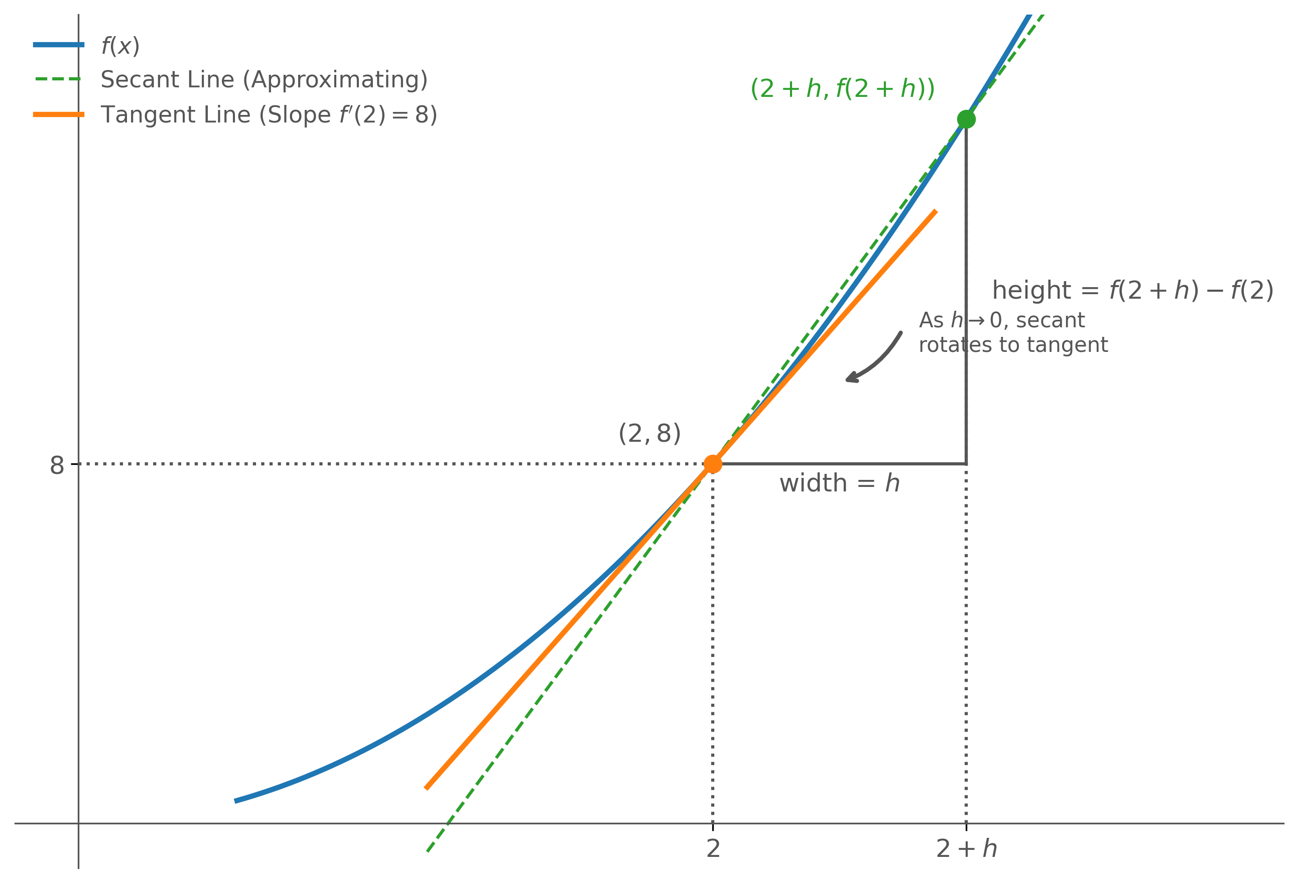
Geometrically, we can also think of the derivative as the limit of the slope of a secant line: a straight line connecting two nearby points on the curve (from to ).
As the second point is brought closer to the first (meaning ), the secant line rotates downward until it perfectly coincides with the tangent line. This visual rotation is exactly what the formal limit definition represents:
Why Numerical Methods are Needed
Analytical differentiation works perfectly when is available as an explicit formula. In practice, that is not always possible:
- is defined only by a table of measured data points, with no underlying formula.
- is so complex that computing its derivative analytically is impractical.
- The function is the output of a simulation or physical measurement.
In all of these cases, we use numerical differentiation: approximating the derivative using only a discrete set of function values . The key idea is that the secant slope between two points close to is a good approximation of the tangent slope at . The smaller the gap between the two points, the better the approximation.