Bisection Method

The bisection method is the most straightforward root-finding algorithm. It works by repeatedly halving an interval that is guaranteed to contain a root, narrowing in on the solution with each step. While not the fastest method, it is unconditionally convergent whenever its starting condition is satisfied.

---

The Sign-Change Condition

If a continuous function changes sign over an interval $[a, b]$, then by the Intermediate Value Theorem it must cross the x-axis at least once inside that interval.

$f(a) \cdot f(b) < 0 \implies \text{a root exists in } [a, b]$

Conversely, if $f(a) \cdot f(b) > 0$, both endpoints have the same sign and the method cannot be applied to that interval.

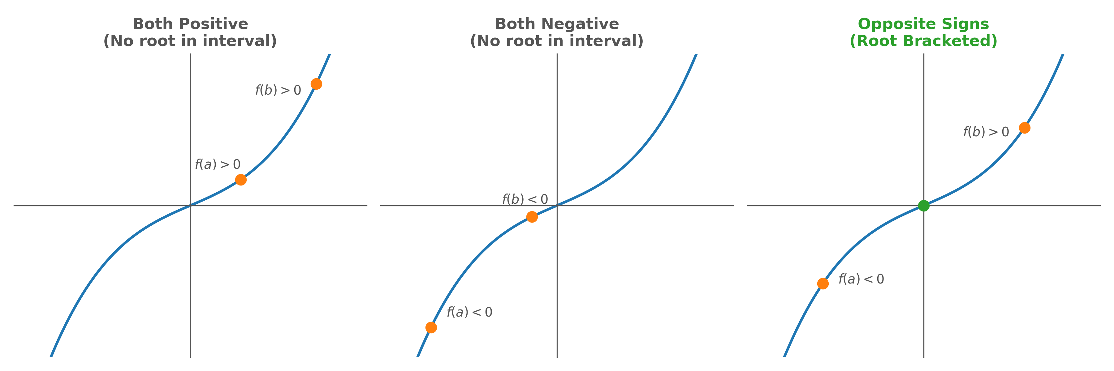
As seen in the figure above, when we choose an interval where the function values at the boundaries share the same sign (both positive or both negative), there is no guarantee that the function crosses the zero axis within that specific window. We must bracket the root by finding one positive and one negative point.

Note

The sign-change condition guarantees at least one root in $[a, b]$, but not uniqueness. If there are two roots, the product $f(a) \cdot f(b)$ could be positive even though roots exist. Bisection finds one root per interval, so it is common practice to bracket roots individually.

---

Algorithm

At each iteration $k$, compute the midpoint $m_k$ and evaluate the function there:

$m_k = \frac{a_k + b_k}{2}$

Then update the interval by checking the signs. The algorithm strictly follows one of three paths:

• Left Half: If $f(a_k) \cdot f(m_k) < 0$, the root lies between $a_k$ and $m_k$. Set $b_{k+1} = m_k$.
• Right Half: If $f(m_k) \cdot f(b_k) < 0$, the root lies between $m_k$ and $b_k$. Set $a_{k+1} = m_k$.
• Exact Root: If $f(m_k) = 0$, then $m_k$ is the root exactly, and the algorithm halts.

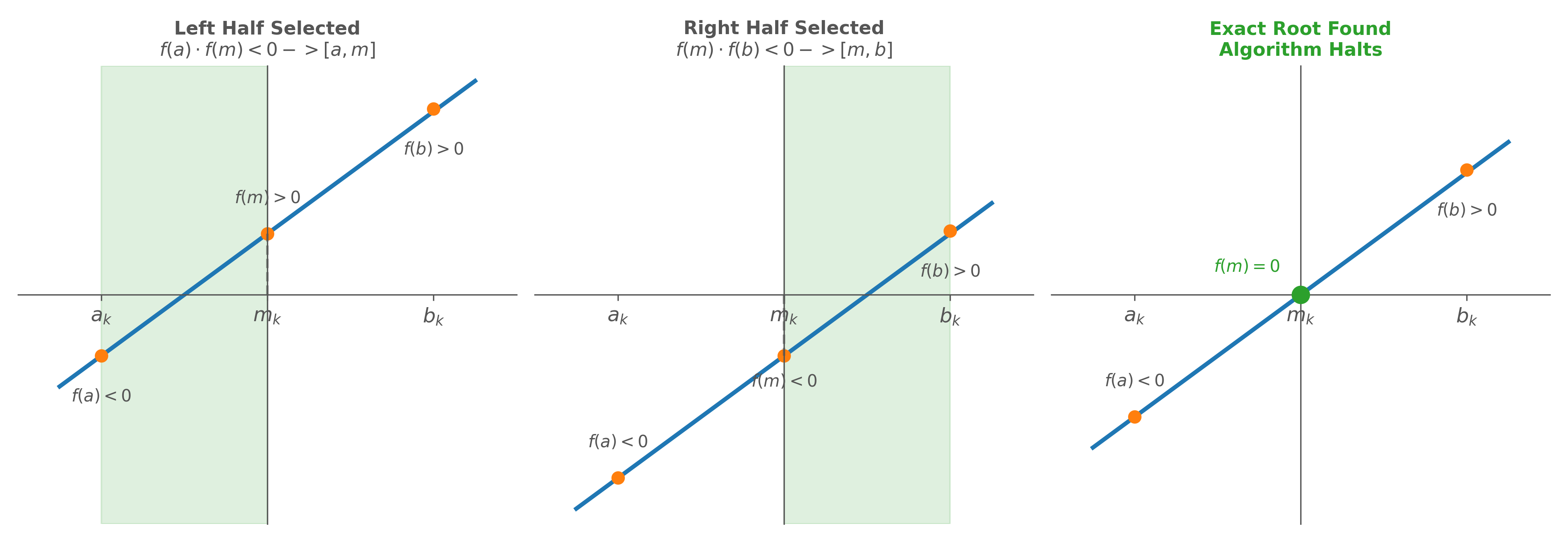
By replacing one of the boundaries with the midpoint, the interval length halves after every single iteration:

$|b_k - a_k| = \frac{|b_0 - a_0|}{2^k}$

---

Minimum Number of Iterations

Formula

Given an initial interval $[a_0, b_0]$ and an error tolerance $\epsilon$, the minimum number of iterations $n$ required is:

$n \ge \frac{\log|b_0 - a_0| - \log \epsilon}{\log 2} - 1$

Proof

After $k$ iterations, the interval has length $\dfrac{|b_0 - a_0|}{2^k}$. The midpoint $m_k$ is at most half an interval-width away from the true root $x^*$ (the worst case is when $x^*$ sits at one of the endpoints $a_k$ or $b_k$):

$|m_k - x^*| \le \frac{|b_k - a_k|}{2} = \frac{|b_0 - a_0|}{2^{k+1}}$

For the error to fall within tolerance $\epsilon$ after $n$ iterations:

$\frac{|b_0 - a_0|}{2^{n+1}} \le \epsilon$

Taking logarithms of both sides:

$\log|b_0 - a_0| - (n+1)\log 2 \le \log \epsilon$

$\log|b_0 - a_0| - n\log 2 - \log 2 \le \log \epsilon$

$n\log 2 \ge \log|b_0 - a_0| - \log \epsilon - \log 2$

$\boxed{n \ge \frac{\log|b_0 - a_0| - \log \epsilon}{\log 2} - 1}$

---

Worked Example 1: Minimum Iterations

Problem: Given interval $[1.5,\; 3]$ and machine epsilon $\epsilon_M = 1.1 \times 10^{-16}$, find the minimum number of bisection iterations required.

Step 1 — Identify the inputs

$a_0 = 1.5, \quad b_0 = 3, \quad \epsilon = 1.1 \times 10^{-16}$

$|b_0 - a_0| = |3 - 1.5| = 1.5$

Step 2 — Apply the formula

$n \ge \frac{\log(1.5) - \log(1.1 \times 10^{-16})}{\log(2)} - 1 \approx 52.59$

Step 3 — Round up

Since $n$ must be an integer:

$\boxed{n = 53 \text{ iterations}}$

---

Worked Example 2: Running Bisection

Problem: Use the bisection method to find the root of $f(x) = x^3 - 7x^2 + 14x - 6$ on $[1,\; 3.2]$ accurate within $10^{-3}$.

Step 1 — Verify the sign-change condition

$f(1) = 1 - 7 + 14 - 6 = 2 \quad (> 0)$

$f(3.2) = (3.2)^3 - 7(3.2)^2 + 14(3.2) - 6 = 32.768 - 71.68 + 44.8 - 6 = -0.112 \quad (< 0)$

Since $f(1) \cdot f(3.2) < 0$, a root exists in $[1,\; 3.2]$.

Step 2 — Iterate

At each step, compute the midpoint and decide which half contains the root. The table below shows 10 iterations:

$k$	$a_k$	$m_k$	$b_k$	$f(a_k)$	$f(m_k)$	$f(b_k)$
0	1.000000	2.100000	3.200000	2.000000	1.791000	$-$0.112000
1	2.100000	2.650000	3.200000	1.791000	0.552125	$-$0.112000
2	2.650000	2.925000	3.200000	0.552125	0.085828	$-$0.112000
3	2.925000	3.062500	3.200000	0.085828	$-$0.054443	$-$0.112000
4	2.925000	2.993750	3.062500	0.085828	0.006328	$-$0.054443
5	2.993750	3.028125	3.062500	0.006328	$-$0.026521	$-$0.054443
6	2.993750	3.010938	3.028125	0.006328	$-$0.010697	$-$0.026521
7	2.993750	3.002344	3.010938	0.006328	$-$0.002333	$-$0.010697
8	2.993750	2.998047	3.002344	0.006328	0.001961	$-$0.002333
9	2.998047	3.000195	3.002344	0.001961	$-$0.000195	$-$0.002333

Step 3 — Read the result

At iteration 9, the midpoint is $m_9 = 3.000195$ and $|f(m_9)| = 0.000195 < 10^{-3}$. The method has converged.

$\boxed{x^* \approx 3.000}$