Runge's Phenomenon & Chebyshev Nodes

Everything covered so far suggests a simple strategy: more nodes → higher degree → smaller error. For well-behaved functions this holds true. But for certain functions, increasing the number of equally spaced nodes does not reduce the error — it makes things catastrophically worse. This failure mode is called Runge’s phenomenon, and Chebyshev nodes are the elegant, principled remedy.

---

The Problem — Runge’s Phenomenon

Consider the function:

$f(x) = \frac{1}{1 + 25x^2}, \qquad x \in [-1, 1]$

If we interpolate using equally spaced nodes and keep adding more, something unexpected happens: the polynomial stays close to $f(x)$ near the centre of the interval, but enormous oscillating spikes appear near the endpoints $x = -1$ and $x = 1$. As $n \to \infty$, the error at the endpoints grows without bound — the interpolation diverges precisely where you’d expect it to converge.

Caution

This means the naive strategy of “just use more equally spaced nodes” can actively make things worse. The error formula explains why: even though $\frac{\max|f^{(n+1)}(\xi)|}{(n+1)!}$ shrinks, the node product $|W(x)|$ at the endpoints grows faster. $|W(x)|$ wins, and the bound blows up.

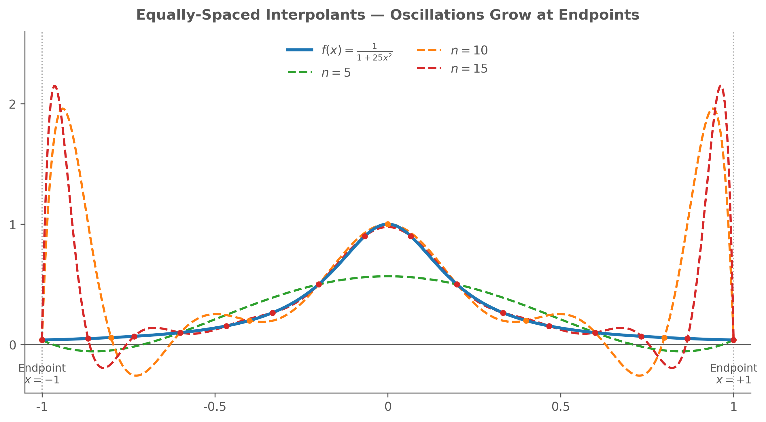
Causes

Runge’s phenomenon arises from two interacting factors:

1. The function itself — Functions with poles or rapid variation near (but outside) the interval are especially susceptible. The function $\frac{1}{1+25x^2}$ has complex poles at $x = \pm \frac{i}{5}$, which sit very close to the real interval in the complex plane. This forces the polynomial to “chase” a sharp feature it cannot fully capture.

2. Equally spaced nodes — With uniform spacing, the outermost nodes are relatively far from the endpoints of the interval. The product $|W(x)|$ at the boundaries — where no nodes are present to “anchor” the polynomial — grows unchecked as $n$ increases.

---

Solutions

Because the error spikes at the boundaries, the fix is to concentrate more nodes near the endpoints. Two strategies accomplish this:

1. Piecewise Interpolation

Divide $[a,b]$ into smaller sub-intervals and build a low-degree polynomial on each piece, then stitch the pieces together. Each segment is short enough that $|W(x)|$ stays small throughout, and oscillations from one piece cannot propagate to another.

2. Chebyshev Nodes

Rather than splitting the interval, choose a smarter set of node positions across the full interval. Chebyshev nodes cluster naturally near the boundaries and are mathematically proven to minimise $\max_{x \in [a,b]}|W(x)|$ among all possible choices of $n+1$ nodes — making them the optimal antidote to Runge’s phenomenon.

---

Chebyshev Nodes — The Semicircle Intuition

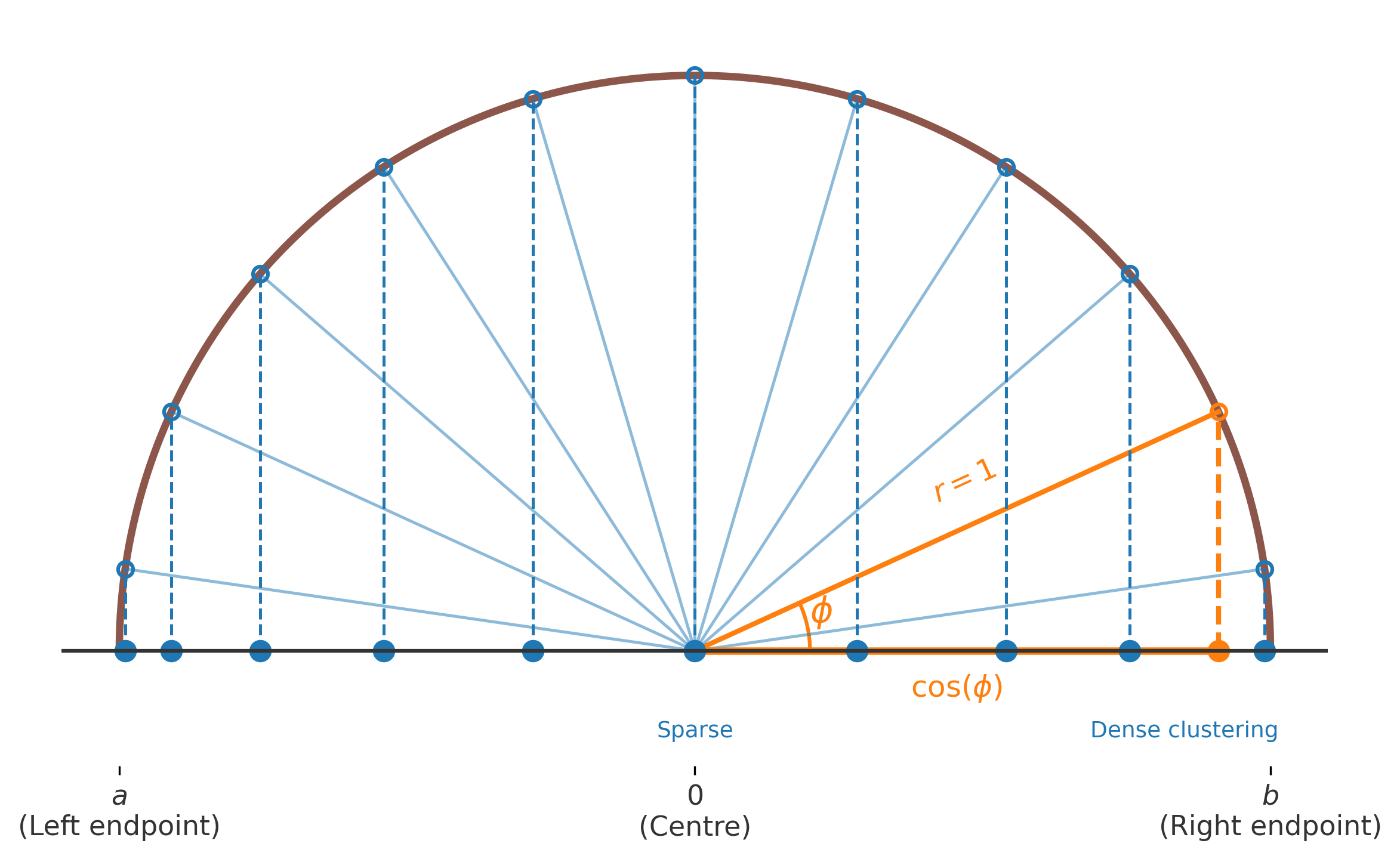
Imagine the interval $[a,b]$ as the diameter of a semicircle of radius $r = \frac{b-a}{2}$ centred at $c = \frac{a+b}{2}$.

Place $n+1$ equally spaced points along the arc (circumference) of the semicircle — governed by an angle $\phi$. To find the position on the interval, we project each arc point vertically downward onto the diameter using the cosine function.

The Role of Cosine

The angle $\phi$ spaces the points evenly along the curved arc. But we only care about their horizontal position on the diameter, which is governed by $\cos(\phi)$.

• Near the middle: When $\phi$ is near $\frac{\pi}{2}$ (the top of the arc), the cosine function changes rapidly. Points projected from here are spaced far apart.
• Near the endpoints: When $\phi$ is near $0$ or $\pi$ (the edges of the arc), the cosine function flattens out. A large change in the angle $\phi$ results in only a tiny change in the horizontal $\cos(\phi)$ value.

This trigonometric property naturally creates the optimal distribution: dense near the endpoints and sparse in the middle, perfectly suppressing $|W(x)|$ at the boundaries.

Therefore, for an interval centered at the origin (like the one in our figure), we can express the Chebyshev nodes explicitly as:

$x_j = r\cos(\phi_j), \qquad j = 0, 1, \ldots, n$

where the angles $\phi_j$ space the $n+1$ points evenly along the arc.

To generalize this for an arbitrary interval $[a,b]$, we simply scale the radius to match the interval’s width and shift the semicircle so it aligns with the interval’s centre, $c$. The general node positions become:

$x_j = r\cos(\phi_j) + c, \qquad j = 0, 1, \ldots, n$

where each component directly reflects our geometric model:

• $r = \frac{b-a}{2}$ (Radius): Scales the unit circle to match the exact half-width of the target interval.
• $c = \frac{a+b}{2}$ (Centre): Shifts the semicircle along the number line so its midpoint aligns with the interval’s centre.
• $\phi_j = \frac{(2j+1)\pi}{2(n+1)}$ (Angle): Defines the evenly spaced angular positions of the $n+1$ nodes along the arc.

Working together, the angles $\phi_j$ guarantee a uniform distribution along the curve, while the $\cos(\phi_j)$ factor executes the crucial vertical projection down to the x-axis—naturally creating the boundary-heavy clustering required to minimize oscillation.

---

Note

Chebyshev nodes do not eliminate interpolation error — they minimise it in the minimax sense. Among all possible choices of $n+1$ nodes in $[a,b]$, Chebyshev nodes are the unique configuration that minimises $\max_{x \in [a,b]} |W(x)|$.

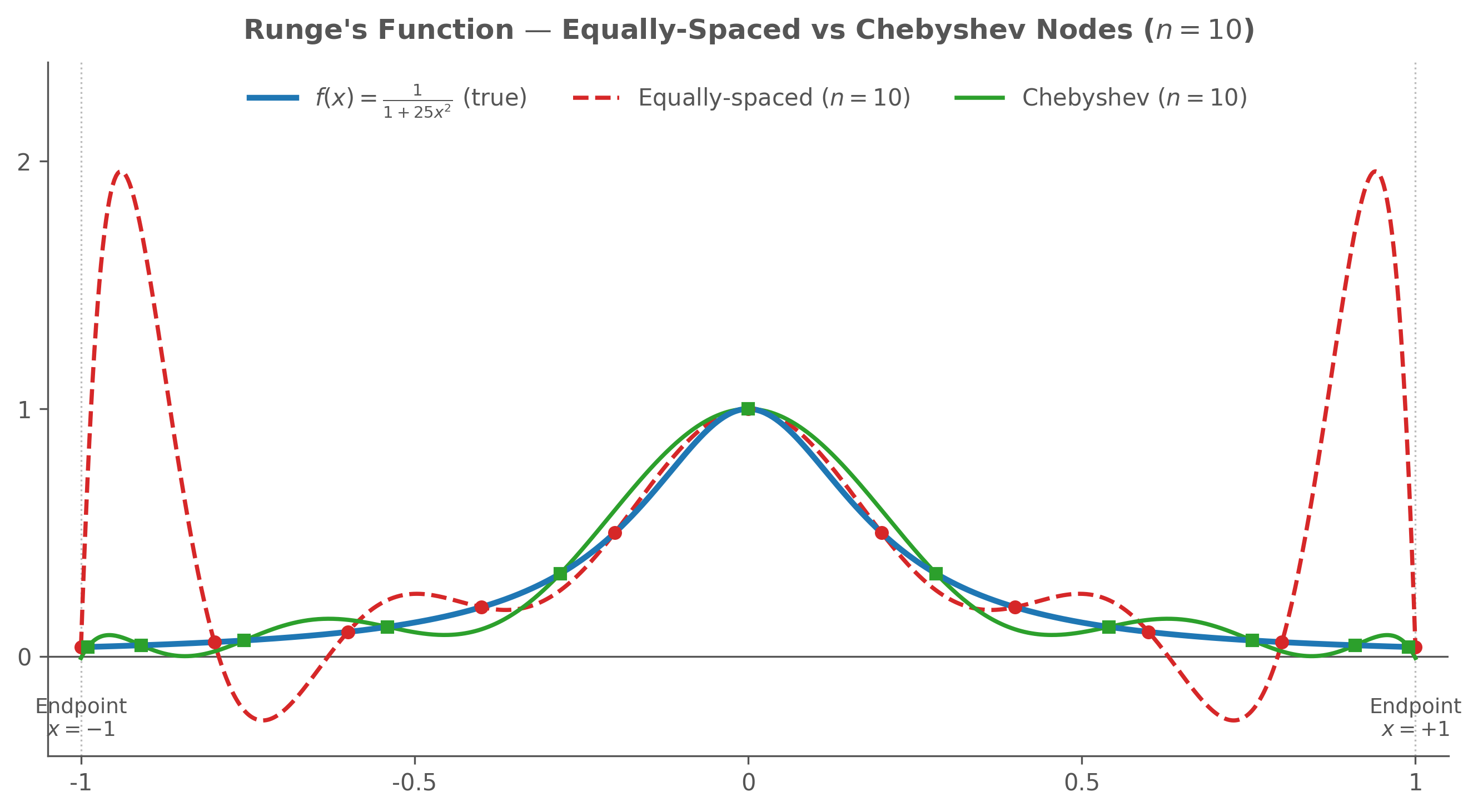
The figure below makes this concrete for the Runge function. Both strategies target $f(x) = \frac{1}{1+25x^2}$ on $[-1,1]$; only the node placement differs.

Worked Example

Problem: Find the 4 Chebyshev nodes for a degree-3 polynomial on the interval $[2, 6]$.

Parameter	Value
Interval $[a,b]$	$[2,\ 6]$
Degree $n$	$3$
Nodes required	$4$

$r = \frac{6-2}{2} = 2, \qquad c = \frac{6+2}{2} = 4$

Angles (for $j = 0, 1, 2, 3$ with $n+1 = 4$):

$j$	$\phi_j = \dfrac{(2j+1)\pi}{8}$	$\cos(\phi_j)$	$x_j = 2\cos(\phi_j) + 4$
0	$\dfrac{\pi}{8}$	$0.9239$	$5.848$
1	$\dfrac{3\pi}{8}$	$0.3827$	$4.765$
2	$\dfrac{5\pi}{8}$	$-0.3827$	$3.235$
3	$\dfrac{7\pi}{8}$	$-0.9239$	$2.152$

The four Chebyshev nodes are approximately:

$x_0 \approx 5.848, \quad x_1 \approx 4.765, \quad x_2 \approx 3.235, \quad x_3 \approx 2.152$

Notice the distribution: two nodes sit close to each endpoint (near 2 and near 6), while the middle of the interval is more sparsely covered. This clustering is exactly what prevents the boundary oscillations characteristic of Runge’s phenomenon.