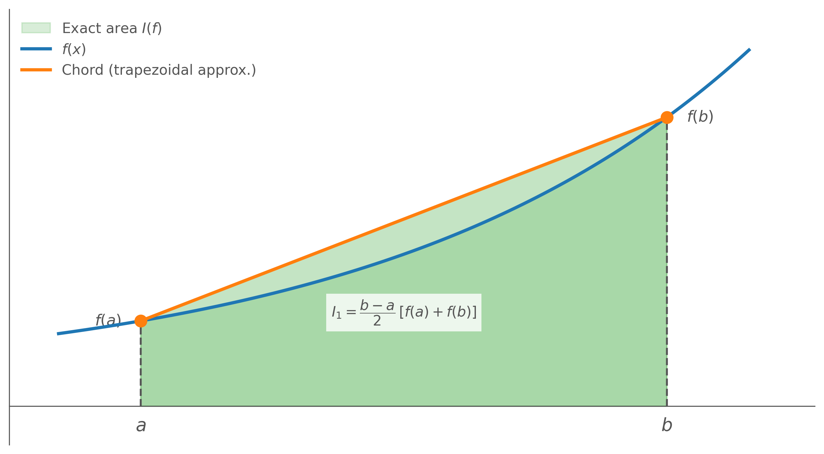
The Trapezoidal Rule is the simplest closed Newton-Cotes formula. It uses two nodes: the left endpoint x0=a and the right endpoint x1=b. The integrand is approximated by the straight line connecting f(a) and f(b), and the integral of that line is the area of a trapezoid.
The chord either overestimates or underestimates depending on the curvature of f(x); the derivation below computes the weights σ0 and σ1 that make this approximation exact.
We compute each weight by integrating its basis polynomial over [a,b].
Derivation of σ0
σ0=∫abl0(x)dx=∫aba−bx−bdx=a−b1∫ab(x−b)dx
Evaluating the integral:
=a−b1[2x2−bx]ab
=a−b1(2b2−b2−2a2+ab)
=a−b1⋅2b2−2b2−a2+2ab
=a−b1⋅2−(b2−2ab+a2)
=a−b1⋅2−(b−a)2
Since a−b=−(b−a):
σ0=−(b−a)1⋅2−(b−a)2=2b−a
Derivation of σ1
σ1=∫abl1(x)dx=∫abb−ax−adx=b−a1∫ab(x−a)dx
Evaluating the integral:
=b−a1[2x2−ax]ab
=b−a1(2b2−ab−2a2+a2)
=b−a1⋅2b2−2ab+a2
=b−a1⋅2(b−a)2=2b−a
The Trapezoidal Rule
Both weights are equal:
σ0=σ1=2b−a
Substituting back:
I1=2b−a[f(a)+f(b)]
Geometric Interpretation
The Trapezoidal Rule replaces the curved region under f(x) with a trapezoid. The two parallel sides of the trapezoid have heights f(a) and f(b), and the perpendicular distance between them is b−a:
Area of trapezoid=21(b−a)[f(a)+f(b)]
For smooth functions that are nearly linear over [a,b], the trapezoidal approximation is quite good. When the function curves significantly, the approximation can be far off. The Composite Trapezoidal Rule (next section) addresses this by breaking the interval into many small sub-intervals, each of which is nearly linear.
The factor of 21 in the formula comes directly from the geometry: the area of any trapezoid is half the sum of its parallel sides multiplied by the perpendicular distance between them.
![A labeled trapezoid with parallel sides f(a) and f(b), base b minus a, and the area formula (b-a)/2 times [f(a)+f(b)] displayed inside.](/images/numerical-integration/trapezoidal-trapezoid.png)