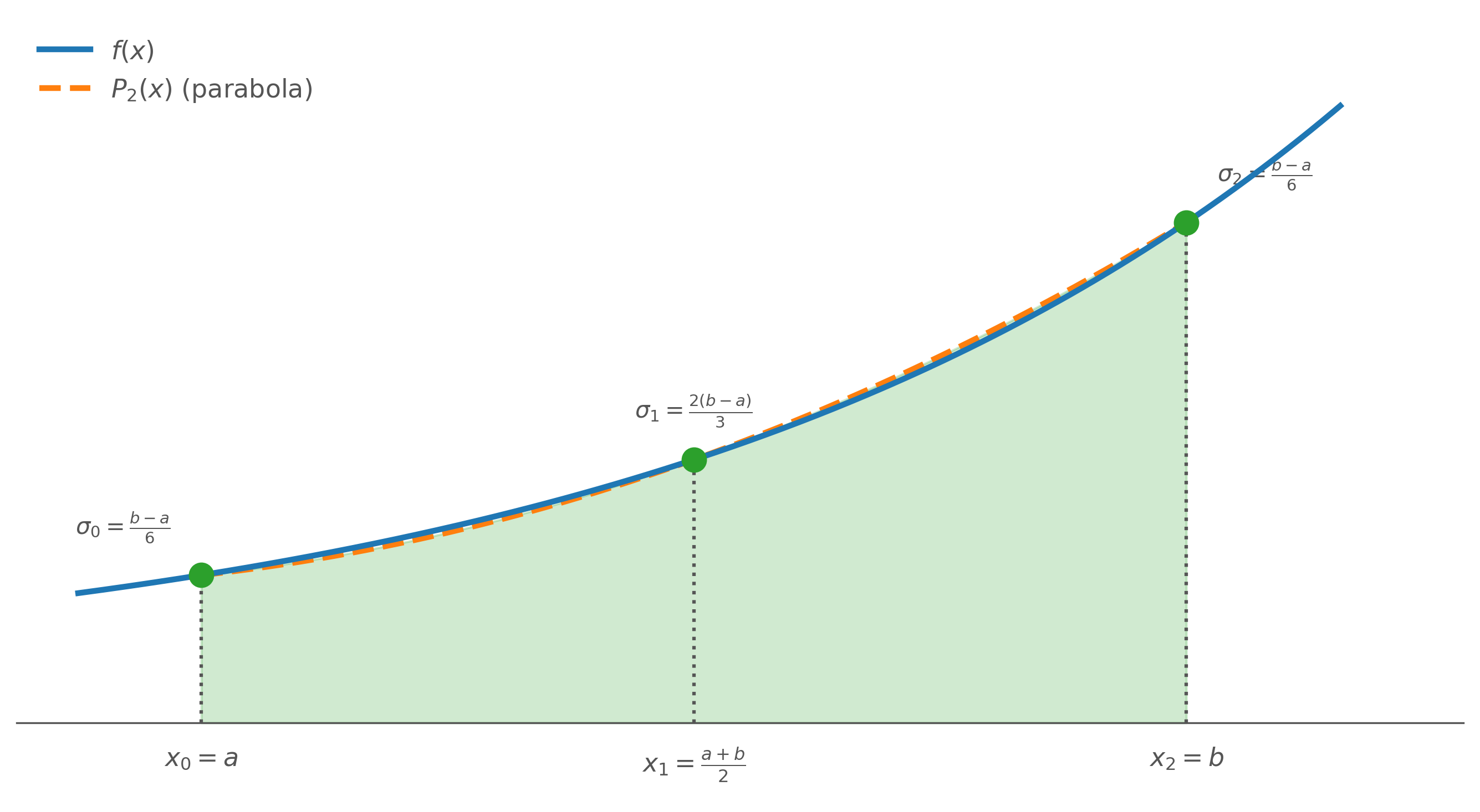
Simpson’s Rule is the closed Newton-Cotes formula for n = 2 n = 2 n = 2
The parabola matches f ( x ) f(x) f ( x ) σ k \sigma_k σ k
Setup
For n = 2 n = 2 n = 2
Node x x x f f f x 0 x_0 x 0 a a a f ( a ) f(a) f ( a ) x 1 x_1 x 1 a + b 2 \dfrac{a+b}{2} 2 a + b f ( a + b 2 ) f\!\left(\dfrac{a+b}{2}\right) f ( 2 a + b ) x 2 x_2 x 2 b b b f ( b ) f(b) f ( b )
The Newton-Cotes formula gives:
I 2 = σ 0 f ( x 0 ) + σ 1 f ( x 1 ) + σ 2 f ( x 2 ) I_2 = \sigma_0\, f(x_0) + \sigma_1\, f(x_1) + \sigma_2\, f(x_2) I 2 = σ 0 f ( x 0 ) + σ 1 f ( x 1 ) + σ 2 f ( x 2 )
We compute each weight σ k = ∫ a b l k ( x ) d x \sigma_k = \int_a^b l_k(x)\,dx σ k = ∫ a b l k ( x ) d x
Derivation of σ 0 \sigma_0 σ 0
σ 0 = ∫ a b l 0 ( x ) d x = ∫ a b ( x − x 1 ) ( x − x 2 ) ( x 0 − x 1 ) ( x 0 − x 2 ) d x \sigma_0 = \int_a^b l_0(x)\,dx = \int_a^b \frac{(x - x_1)(x - x_2)}{(x_0 - x_1)(x_0 - x_2)}\,dx σ 0 = ∫ a b l 0 ( x ) d x = ∫ a b ( x 0 − x 1 ) ( x 0 − x 2 ) ( x − x 1 ) ( x − x 2 ) d x
Substituting the node values:
= ∫ a b ( x − a + b 2 ) ( x − b ) ( a − a + b 2 ) ( a − b ) d x = \int_a^b \frac{\left(x - \tfrac{a+b}{2}\right)(x - b)}{\left(a - \tfrac{a+b}{2}\right)(a - b)}\,dx = ∫ a b ( a − 2 a + b ) ( a − b ) ( x − 2 a + b ) ( x − b ) d x
The denominator factors simplify: a − a + b 2 = a − b 2 a - \tfrac{a+b}{2} = \tfrac{a-b}{2} a − 2 a + b = 2 a − b ( a − a + b 2 ) ( a − b ) = ( a − b ) 2 2 (a - \tfrac{a+b}{2})(a-b) = \tfrac{(a-b)^2}{2} ( a − 2 a + b ) ( a − b ) = 2 ( a − b ) 2 x − a + b 2 = 2 x − a − b 2 x - \tfrac{a+b}{2} = \tfrac{2x-a-b}{2} x − 2 a + b = 2 2 x − a − b
= ∫ a b ( 2 x − a − b ) 2 ( x − b ) ( a − b ) 2 2 d x = 1 ( a − b ) 2 ∫ a b ( 2 x − a − b ) ( x − b ) d x = \int_a^b \frac{\tfrac{(2x-a-b)}{2}(x-b)}{\tfrac{(a-b)^2}{2}}\,dx = \frac{1}{(a-b)^2}\int_a^b (2x-a-b)(x-b)\,dx = ∫ a b 2 ( a − b ) 2 2 ( 2 x − a − b ) ( x − b ) d x = ( a − b ) 2 1 ∫ a b ( 2 x − a − b ) ( x − b ) d x
Expanding the integrand:
= 1 ( a − b ) 2 ∫ a b ( 2 x 2 − a x − b x − 2 b x + a b + b 2 ) d x = \frac{1}{(a-b)^2}\int_a^b \left(2x^2 - ax - bx - 2bx + ab + b^2\right)dx = ( a − b ) 2 1 ∫ a b ( 2 x 2 − a x − b x − 2 b x + ab + b 2 ) d x
Integrating term by term:
= 1 ( a − b ) 2 [ 2 x 3 3 − a x 2 2 − b x 2 2 − b x 2 + a b x + b 2 x ] a b = \frac{1}{(a-b)^2}\left[\frac{2x^3}{3} - \frac{ax^2}{2} - \frac{bx^2}{2} - bx^2 + abx + b^2 x\right]_a^b = ( a − b ) 2 1 [ 3 2 x 3 − 2 a x 2 − 2 b x 2 − b x 2 + ab x + b 2 x ] a b
Evaluating at both limits and writing the combined expression:
= 1 ( a − b ) 2 ( 2 b 3 3 − a b 2 2 − b 3 2 − b 3 + a b 2 + b 3 − 2 a 3 3 + a 3 2 + a 2 b 2 + a 2 b − a 2 b − a b 2 ) = \frac{1}{(a-b)^2}\left(\frac{2b^3}{3} - \frac{ab^2}{2} - \frac{b^3}{2} - b^3 + ab^2 + b^3 - \frac{2a^3}{3} + \frac{a^3}{2} + \frac{a^2b}{2} + a^2b - a^2b - ab^2\right) = ( a − b ) 2 1 ( 3 2 b 3 − 2 a b 2 − 2 b 3 − b 3 + a b 2 + b 3 − 3 2 a 3 + 2 a 3 + 2 a 2 b + a 2 b − a 2 b − a b 2 )
Collecting like terms:
= 1 ( a − b ) 2 ( 2 b 3 3 − 2 a 3 3 + a 3 2 − b 3 2 + a 2 b 2 − a b 2 2 ) = \frac{1}{(a-b)^2}\left(\frac{2b^3}{3} - \frac{2a^3}{3} + \frac{a^3}{2} - \frac{b^3}{2} + \frac{a^2b}{2} - \frac{ab^2}{2}\right) = ( a − b ) 2 1 ( 3 2 b 3 − 3 2 a 3 + 2 a 3 − 2 b 3 + 2 a 2 b − 2 a b 2 )
Converting to a common denominator of 144:
= 1 ( a − b ) 2 ⋅ 96 b 3 − 96 a 3 + 72 a 3 − 72 b 3 + 72 a 2 b − 72 a b 2 144 = \frac{1}{(a-b)^2} \cdot \frac{96b^3 - 96a^3 + 72a^3 - 72b^3 + 72a^2b - 72ab^2}{144} = ( a − b ) 2 1 ⋅ 144 96 b 3 − 96 a 3 + 72 a 3 − 72 b 3 + 72 a 2 b − 72 a b 2
= 1 ( a − b ) 2 ⋅ 24 b 3 − 24 a 3 + 72 a 2 b − 72 a b 2 144 = \frac{1}{(a-b)^2} \cdot \frac{24b^3 - 24a^3 + 72a^2 b - 72ab^2}{144} = ( a − b ) 2 1 ⋅ 144 24 b 3 − 24 a 3 + 72 a 2 b − 72 a b 2
= 1 ( a − b ) 2 ⋅ 24 ( b 3 − a 3 + 3 a 2 b − 3 a b 2 ) 144 = \frac{1}{(a-b)^2} \cdot \frac{24\bigl(b^3 - a^3 + 3a^2 b - 3ab^2\bigr)}{144} = ( a − b ) 2 1 ⋅ 144 24 ( b 3 − a 3 + 3 a 2 b − 3 a b 2 )
Recognizing that b 3 − a 3 + 3 a 2 b − 3 a b 2 = ( b − a ) 3 b^3 - a^3 + 3a^2b - 3ab^2 = (b-a)^3 b 3 − a 3 + 3 a 2 b − 3 a b 2 = ( b − a ) 3
σ 0 = 1 ( b − a ) 2 ⋅ ( b − a ) 3 6 = b − a 6 \sigma_0 = \frac{1}{(b-a)^2} \cdot \frac{(b-a)^3}{6} = \frac{b-a}{6} σ 0 = ( b − a ) 2 1 ⋅ 6 ( b − a ) 3 = 6 b − a
Derivation of σ 1 \sigma_1 σ 1
σ 1 = ∫ a b l 1 ( x ) d x = ∫ a b ( x − x 0 ) ( x − x 2 ) ( x 1 − x 0 ) ( x 1 − x 2 ) d x \sigma_1 = \int_a^b l_1(x)\,dx = \int_a^b \frac{(x - x_0)(x - x_2)}{(x_1 - x_0)(x_1 - x_2)}\,dx σ 1 = ∫ a b l 1 ( x ) d x = ∫ a b ( x 1 − x 0 ) ( x 1 − x 2 ) ( x − x 0 ) ( x − x 2 ) d x
The denominator factors are x 1 − x 0 = b − a 2 x_1 - x_0 = \tfrac{b-a}{2} x 1 − x 0 = 2 b − a x 1 − x 2 = a − b 2 x_1 - x_2 = \tfrac{a-b}{2} x 1 − x 2 = 2 a − b − ( b − a ) 2 4 -\tfrac{(b-a)^2}{4} − 4 ( b − a ) 2
σ 1 = − 4 ( b − a ) 2 ∫ a b ( x − a ) ( x − b ) d x \sigma_1 = \frac{-4}{(b-a)^2}\int_a^b (x-a)(x-b)\,dx σ 1 = ( b − a ) 2 − 4 ∫ a b ( x − a ) ( x − b ) d x
Expanding the integrand:
= − 4 ( b − a ) 2 ∫ a b ( x 2 − a x − b x + a b ) d x = \frac{-4}{(b-a)^2}\int_a^b \left(x^2 - ax - bx + ab\right)dx = ( b − a ) 2 − 4 ∫ a b ( x 2 − a x − b x + ab ) d x
Integrating term by term:
= − 4 ( b − a ) 2 [ x 3 3 − a x 2 2 − b x 2 2 + a b x ] a b = \frac{-4}{(b-a)^2}\left[\frac{x^3}{3} - \frac{ax^2}{2} - \frac{bx^2}{2} + abx\right]_a^b = ( b − a ) 2 − 4 [ 3 x 3 − 2 a x 2 − 2 b x 2 + ab x ] a b
Evaluating at both limits and writing the combined expression:
= − 4 ( b − a ) 2 ( b 3 3 − a b 2 2 − b 3 2 + a b 2 − a 3 3 + a 3 2 + a 2 b 2 − a 2 b ) = \frac{-4}{(b-a)^2}\left(\frac{b^3}{3} - \frac{ab^2}{2} - \frac{b^3}{2} + ab^2 - \frac{a^3}{3} + \frac{a^3}{2} + \frac{a^2b}{2} - a^2b\right) = ( b − a ) 2 − 4 ( 3 b 3 − 2 a b 2 − 2 b 3 + a b 2 − 3 a 3 + 2 a 3 + 2 a 2 b − a 2 b )
Converting to a common denominator of 144:
= − 4 ( b − a ) 2 ⋅ 48 b 3 − 72 a b 2 − 72 b 3 + 144 a b 2 − 48 a 3 + 72 a 3 + 72 a 2 b − 144 a 2 b 144 = \frac{-4}{(b-a)^2} \cdot \frac{48b^3 - 72ab^2 - 72b^3 + 144ab^2 - 48a^3 + 72a^3 + 72a^2b - 144a^2b}{144} = ( b − a ) 2 − 4 ⋅ 144 48 b 3 − 72 a b 2 − 72 b 3 + 144 a b 2 − 48 a 3 + 72 a 3 + 72 a 2 b − 144 a 2 b
= − 4 ( b − a ) 2 ⋅ − 24 b 3 + 24 a 3 + 72 a b 2 − 72 a 2 b 144 = \frac{-4}{(b-a)^2} \cdot \frac{-24b^3 + 24a^3 + 72ab^2 - 72a^2b}{144} = ( b − a ) 2 − 4 ⋅ 144 − 24 b 3 + 24 a 3 + 72 a b 2 − 72 a 2 b
= − 4 ( b − a ) 2 ⋅ 24 ( a 3 − b 3 − 3 a 2 b + 3 a b 2 ) 144 = \frac{-4}{(b-a)^2} \cdot \frac{24\bigl(a^3 - b^3 - 3a^2 b + 3ab^2\bigr)}{144} = ( b − a ) 2 − 4 ⋅ 144 24 ( a 3 − b 3 − 3 a 2 b + 3 a b 2 )
Recognizing that a 3 − b 3 − 3 a 2 b + 3 a b 2 = ( a − b ) 3 = − ( b − a ) 3 a^3 - b^3 - 3a^2b + 3ab^2 = (a-b)^3 = -(b-a)^3 a 3 − b 3 − 3 a 2 b + 3 a b 2 = ( a − b ) 3 = − ( b − a ) 3
σ 1 = − 4 ( b − a ) 2 ⋅ − ( b − a ) 3 6 = 4 ( b − a ) 6 = 2 ( b − a ) 3 \sigma_1 = \frac{-4}{(b-a)^2} \cdot \frac{-(b-a)^3}{6} = \frac{4(b-a)}{6} = \frac{2(b-a)}{3} σ 1 = ( b − a ) 2 − 4 ⋅ 6 − ( b − a ) 3 = 6 4 ( b − a ) = 3 2 ( b − a )
Derivation of σ 2 \sigma_2 σ 2
σ 2 = ∫ a b l 2 ( x ) d x = ∫ a b ( x − x 0 ) ( x − x 1 ) ( x 2 − x 0 ) ( x 2 − x 1 ) d x \sigma_2 = \int_a^b l_2(x)\,dx = \int_a^b \frac{(x - x_0)(x - x_1)}{(x_2 - x_0)(x_2 - x_1)}\,dx σ 2 = ∫ a b l 2 ( x ) d x = ∫ a b ( x 2 − x 0 ) ( x 2 − x 1 ) ( x − x 0 ) ( x − x 1 ) d x
The denominator factors are x 2 − x 0 = b − a x_2 - x_0 = b - a x 2 − x 0 = b − a x 2 − x 1 = b − a 2 x_2 - x_1 = \tfrac{b-a}{2} x 2 − x 1 = 2 b − a ( b − a ) 2 2 \tfrac{(b-a)^2}{2} 2 ( b − a ) 2 x − x 1 = 2 x − a − b 2 x - x_1 = \tfrac{2x-a-b}{2} x − x 1 = 2 2 x − a − b
σ 2 = 1 ( b − a ) 2 ∫ a b ( x − a ) ( 2 x − a − b ) d x \sigma_2 = \frac{1}{(b-a)^2}\int_a^b (x-a)(2x-a-b)\,dx σ 2 = ( b − a ) 2 1 ∫ a b ( x − a ) ( 2 x − a − b ) d x
Expanding the integrand:
= 1 ( b − a ) 2 ∫ a b ( 2 x 2 − a x − b x − 2 a x + a 2 + a b ) d x = \frac{1}{(b-a)^2}\int_a^b \left(2x^2 - ax - bx - 2ax + a^2 + ab\right)dx = ( b − a ) 2 1 ∫ a b ( 2 x 2 − a x − b x − 2 a x + a 2 + ab ) d x
Integrating term by term:
= 1 ( b − a ) 2 [ 2 x 3 3 − a x 2 2 − b x 2 2 − a x 2 + a 2 x + a b x ] a b = \frac{1}{(b-a)^2}\left[\frac{2x^3}{3} - \frac{ax^2}{2} - \frac{bx^2}{2} - ax^2 + a^2 x + abx\right]_a^b = ( b − a ) 2 1 [ 3 2 x 3 − 2 a x 2 − 2 b x 2 − a x 2 + a 2 x + ab x ] a b
Evaluating at both limits and writing the combined expression:
= 1 ( b − a ) 2 ( 2 b 3 3 − a b 2 2 − b 3 2 − a b 2 + a 2 b + a b 2 − 2 a 3 3 + a 3 2 + a 2 b 2 + a 3 − a 3 − a 2 b ) = \frac{1}{(b-a)^2}\left(\frac{2b^3}{3} - \frac{ab^2}{2} - \frac{b^3}{2} - ab^2 + a^2b + ab^2 - \frac{2a^3}{3} + \frac{a^3}{2} + \frac{a^2b}{2} + a^3 - a^3 - a^2b\right) = ( b − a ) 2 1 ( 3 2 b 3 − 2 a b 2 − 2 b 3 − a b 2 + a 2 b + a b 2 − 3 2 a 3 + 2 a 3 + 2 a 2 b + a 3 − a 3 − a 2 b )
Collecting like terms:
= 1 ( b − a ) 2 ( 2 b 3 3 − 2 a 3 3 + a 3 2 − b 3 2 − a b 2 2 + a 2 b 2 ) = \frac{1}{(b-a)^2}\left(\frac{2b^3}{3} - \frac{2a^3}{3} + \frac{a^3}{2} - \frac{b^3}{2} - \frac{ab^2}{2} + \frac{a^2b}{2}\right) = ( b − a ) 2 1 ( 3 2 b 3 − 3 2 a 3 + 2 a 3 − 2 b 3 − 2 a b 2 + 2 a 2 b )
Converting to a common denominator of 144:
= 1 ( b − a ) 2 ⋅ 96 b 3 − 96 a 3 + 72 a 3 − 72 b 3 − 72 a b 2 + 72 a 2 b 144 = \frac{1}{(b-a)^2} \cdot \frac{96b^3 - 96a^3 + 72a^3 - 72b^3 - 72ab^2 + 72a^2b}{144} = ( b − a ) 2 1 ⋅ 144 96 b 3 − 96 a 3 + 72 a 3 − 72 b 3 − 72 a b 2 + 72 a 2 b
= 1 ( b − a ) 2 ⋅ 24 b 3 − 24 a 3 − 72 a b 2 + 72 a 2 b 144 = \frac{1}{(b-a)^2} \cdot \frac{24b^3 - 24a^3 - 72ab^2 + 72a^2b}{144} = ( b − a ) 2 1 ⋅ 144 24 b 3 − 24 a 3 − 72 a b 2 + 72 a 2 b
= 1 ( b − a ) 2 ⋅ 24 ( b 3 − a 3 − 3 a b 2 + 3 a 2 b ) 144 = \frac{1}{(b-a)^2} \cdot \frac{24\bigl(b^3 - a^3 - 3ab^2 + 3a^2b\bigr)}{144} = ( b − a ) 2 1 ⋅ 144 24 ( b 3 − a 3 − 3 a b 2 + 3 a 2 b )
Recognizing that b 3 − a 3 − 3 a b 2 + 3 a 2 b = ( b − a ) 3 b^3 - a^3 - 3ab^2 + 3a^2b = (b-a)^3 b 3 − a 3 − 3 a b 2 + 3 a 2 b = ( b − a ) 3
σ 2 = 1 ( b − a ) 2 ⋅ ( b − a ) 3 6 = b − a 6 \sigma_2 = \frac{1}{(b-a)^2} \cdot \frac{(b-a)^3}{6} = \frac{b-a}{6} σ 2 = ( b − a ) 2 1 ⋅ 6 ( b − a ) 3 = 6 b − a
The three weights are:
σ 0 = b − a 6 , σ 1 = 2 ( b − a ) 3 , σ 2 = b − a 6 \sigma_0 = \frac{b-a}{6}, \qquad \sigma_1 = \frac{2(b-a)}{3}, \qquad \sigma_2 = \frac{b-a}{6} σ 0 = 6 b − a , σ 1 = 3 2 ( b − a ) , σ 2 = 6 b − a
Substituting into I 2 = σ 0 f ( x 0 ) + σ 1 f ( x 1 ) + σ 2 f ( x 2 ) I_2 = \sigma_0 f(x_0) + \sigma_1 f(x_1) + \sigma_2 f(x_2) I 2 = σ 0 f ( x 0 ) + σ 1 f ( x 1 ) + σ 2 f ( x 2 )
I 2 = b − a 6 [ f ( a ) + 4 f ( a + b 2 ) + f ( b ) ] \boxed{I_2 = \frac{b-a}{6}\left[f(a) + 4f\!\left(\frac{a+b}{2}\right) + f(b)\right]} I 2 = 6 b − a [ f ( a ) + 4 f ( 2 a + b ) + f ( b ) ]
The coefficients σ 0 : σ 1 : σ 2 \sigma_0 : \sigma_1 : \sigma_2 σ 0 : σ 1 : σ 2 1 : 4 : 1 1 : 4 : 1 1 : 4 : 1 1 1 1 4 4 4 1 1 1
Why Simpson’s Rule is More Accurate
Even though the Trapezoidal Rule and Simpson’s Rule both use the same interval [ a , b ] [a, b] [ a , b ] f ( x ) f(x) f ( x )