Truncation Error

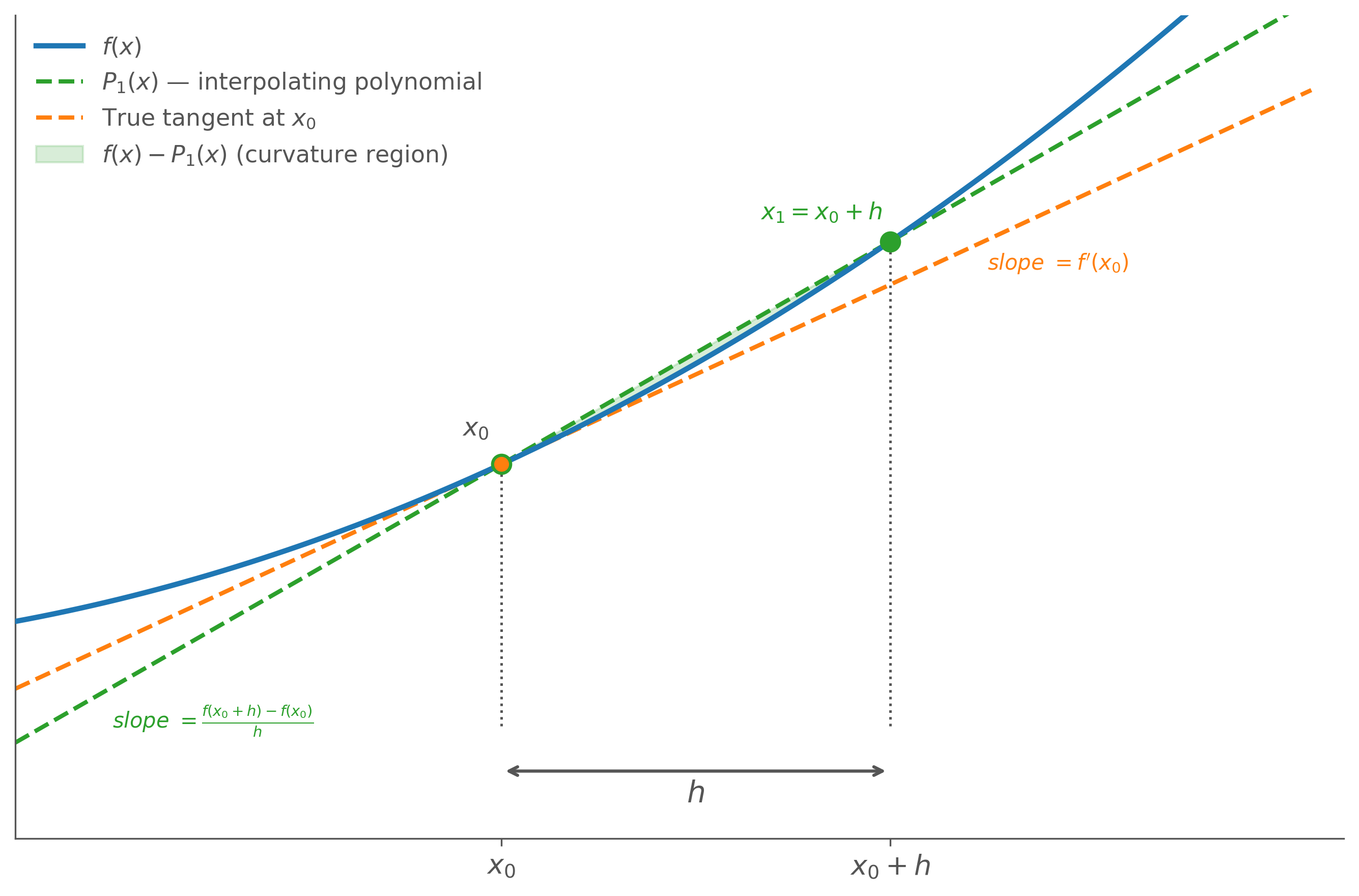
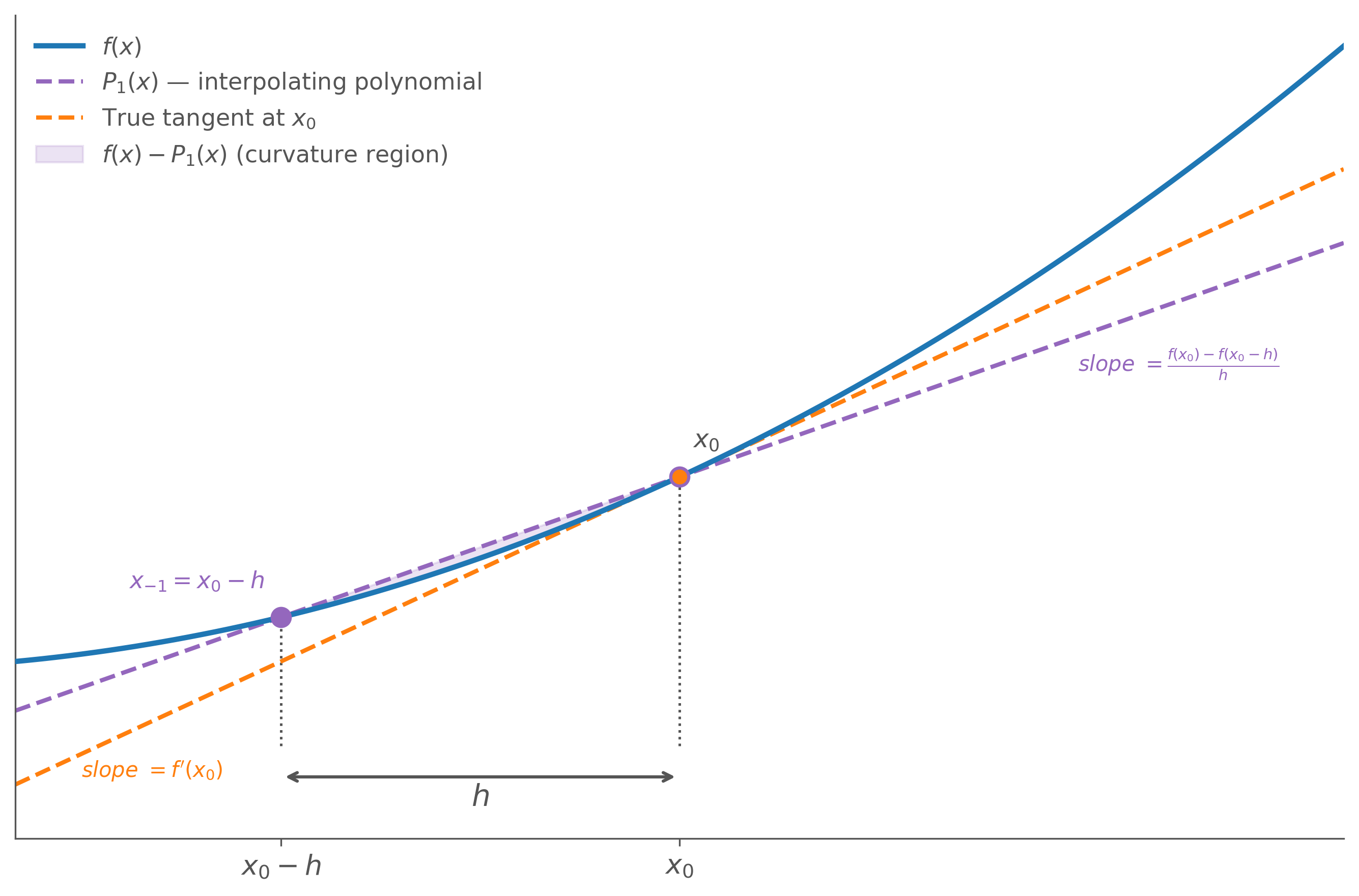
Every numerical derivative is an approximation. The gap between the numerical result and the true derivative is the truncation error, arising because the limiting process $h \to 0$ is replaced by a finite step. By deriving the difference formulas from Taylor or Lagrange series, we can find an explicit expression for this error and compute a bound on its magnitude.

---

Error Orders

The three difference formulas have different error characteristics:

Method	Error Order	Leading Error Term	Effect of dividing $h$ by 10
Forward Difference	$O(h)$	$\dfrac{f''(\xi)}{2}\,h$	Error is divided by 10
Backward Difference	$O(h)$	$\dfrac{f''(\xi)}{2}\,h$	Error is divided by 10
Central Difference	$O(h^2)$	$\dfrac{f'''(\xi)}{6}\,h^2$	Error is divided by 100

For central difference, because the error scales as $h^2$, it shrinks much faster as $h$ decreases. Dividing $h$ by 10 divides the central difference error by 100, whereas the forward and backward errors only halve proportionally with $h$.

Note

The symbol $\xi$ denotes some unknown point inside the interval spanned by the evaluation nodes. We cannot pinpoint it exactly, but we can bound the error by evaluating $|f''(\xi)|$ or $|f'''(\xi)|$ at the point in that interval where it is largest.

---

Proof: Forward Difference Truncation Error

We derive the forward difference formula and its error term using Lagrange interpolation over two nodes: $x_0$ and $x_1 = x_0 + h$.

Setting up the interpolant. Any function $f(x)$ can be written as a first-degree Lagrange polynomial plus an error term:

$f(x) = f(x_0)\frac{x - x_1}{x_0 - x_1} + f(x_1)\frac{x - x_0}{x_1 - x_0} + \frac{f''(\xi)}{2}(x - x_0)(x - x_1)$

Differentiating with respect to $x$:

$f'(x) = \frac{f(x_0)}{x_0 - x_1} + \frac{f(x_1)}{x_1 - x_0} + \frac{f''(\xi)}{2}\frac{d}{dx}\left[(x - x_0)(x - x_1)\right]$

Expanding the derivative of the product in the error term:

$f'(x) = \frac{f(x_0)}{x_0 - x_1} + \frac{f(x_1)}{x_1 - x_0} + \frac{f''(\xi)}{2}(2x - x_0 - x_1)$

Evaluating at $x = x_0$. Since $x_1 - x_0 = h$, we have $x_0 - x_1 = -h$. Substituting $x_1 = x_0 + h$:

$f'(x_0) = \frac{f(x_0)}{-h} + \frac{f(x_1)}{h} + \frac{f''(\xi)}{2}(2x_0 - x_0 - (x_0 + h))$

$f'(x_0) = \frac{f(x_1) - f(x_0)}{h} + \frac{f''(\xi)}{2}(-h)$

$\boxed{f'(x_0) = \underbrace{\frac{f(x_0 + h) - f(x_0)}{h}}_{\text{Forward difference}} - \underbrace{\frac{f''(\xi)}{2}\,h}_{\text{Truncation error}}}$

This confirms two things: the forward difference formula is an exact rearrangement of this identity, and the truncation error is the term $-\frac{f''(\xi)}{2}h$, which is proportional to $h$. Making $h$ smaller reduces this error linearly.

---

Proof: Backward Difference Truncation Error

We can derive the backward difference formula and its error term using Lagrange interpolation over two nodes: $x_0$ and $x_{-1} = x_0 - h$.

Setting up the interpolant. Just like the forward difference, $f(x)$ can be written as a first-degree Lagrange polynomial plus an error term:

$f(x) = f(x_0)\frac{x - x_{-1}}{x_0 - x_{-1}} + f(x_{-1})\frac{x - x_0}{x_{-1} - x_0} + \frac{f''(\xi)}{2}(x - x_0)(x - x_{-1})$

Differentiating with respect to $x$:

$f'(x) = \frac{f(x_0)}{x_0 - x_{-1}} + \frac{f(x_{-1})}{x_{-1} - x_0} + \frac{f''(\xi)}{2}(2x - x_0 - x_{-1})$

Evaluating at $x = x_0$. Since $x_0 - x_{-1} = h$ and $x_{-1} - x_0 = -h$. Substituting $x_{-1} = x_0 - h$:

$f'(x_0) = \frac{f(x_0)}{h} + \frac{f(x_0 - h)}{-h} + \frac{f''(\xi)}{2}(2x_0 - x_0 - (x_0 - h))$

$f'(x_0) = \frac{f(x_0) - f(x_0 - h)}{h} + \frac{f''(\xi)}{2}(h)$

$\boxed{f'(x_0) = \underbrace{\frac{f(x_0) - f(x_0 - h)}{h}}_{\text{Backward difference}} + \underbrace{\frac{f''(\xi)}{2}\,h}_{\text{Truncation error}}}$

The truncation error is proportional to $h$, confirming that backward difference is also an $O(h)$ approximation.

---

Further Reading: Proof of Central Difference Truncation Error

Proof: Central Difference Truncation Error

For the central difference formula, using Taylor series expansions is usually the clearest approach because it naturally reveals how the symmetric terms cancel out.

Setting up the Taylor series. We expand $f(x)$ around $x_0$ to the third degree, evaluating at $x_0 + h$ and $x_0 - h$:

$f(x_0 + h) = f(x_0) + hf'(x_0) + \frac{h^2}{2}f''(x_0) + \frac{h^3}{6}f'''(\xi_1)$

$f(x_0 - h) = f(x_0) - hf'(x_0) + \frac{h^2}{2}f''(x_0) - \frac{h^3}{6}f'''(\xi_2)$

Note

Here, $\xi_1$ is some point in the interval $[x_0, x_0 + h]$ and $\xi_2$ is in $[x_0 - h, x_0]$.

Subtracting the two equations:

$f(x_0 + h) - f(x_0 - h) = 2hf'(x_0) + \frac{h^3}{6}(f'''(\xi_1) + f'''(\xi_2))$

Notice how the $f(x_0)$ and $\frac{h^2}{2}f''(x_0)$ terms completely cancel out.

Consolidating the error term. This step relies on the Intermediate Value Theorem. Think of it like taking an average: $\frac{f'''(\xi_1) + f'''(\xi_2)}{2}$. Because we assume $f'''(x)$ is a continuous function, it must pass through this exact average value at some specific point $\xi$ somewhere between our two outer nodes ($x_0 - h$ and $x_0 + h$).

Mathematically, this means $\frac{f'''(\xi_1) + f'''(\xi_2)}{2} = f'''(\xi)$, which rearranges to $f'''(\xi_1) + f'''(\xi_2) = 2f'''(\xi)$. This allows us to combine the two separate error evaluations into one:

$f(x_0 + h) - f(x_0 - h) = 2hf'(x_0) + \frac{h^3}{6}(2f'''(\xi))$

$f(x_0 + h) - f(x_0 - h) = 2hf'(x_0) + \frac{h^3}{3}f'''(\xi)$

Rearranging to solve for $f'(x_0)$:

$2hf'(x_0) = f(x_0 + h) - f(x_0 - h) - \frac{h^3}{3}f'''(\xi)$

Divide everything by $2h$:

$\boxed{f'(x_0) = \underbrace{\frac{f(x_0 + h) - f(x_0 - h)}{2h}}_{\text{Central difference}} - \underbrace{\frac{f'''(\xi)}{6}\,h^2}_{\text{Truncation error}}}$

Because the $h^2$ terms in the Taylor series perfectly cancelled each other out, the leading error term contains $h^2$. This proves that the central difference method provides an $O(h^2)$ approximation.

Worked Example: Comparing Error Orders

Problem: Approximate the derivative of $f(x) = \ln(x)$ at $x = 2$ using the forward, backward, and central difference formulas with step sizes $h = 0.1, 0.01, 0.001$. Compare the errors with the exact derivative.

The exact derivative is $f'(x) = 1/x$, so at $x = 2$:

$f'(2) = \frac{1}{2} = 0.5$

Step 1 — Compute the numerical derivatives

The three formulas are:

$\text{Forward} = \frac{\ln(2+h) - \ln 2}{h}, \qquad \text{Backward} = \frac{\ln 2 - \ln(2-h)}{h}, \qquad \text{Central} = \frac{\ln(2+h) - \ln(2-h)}{2h}$

The approximations are:

$h$	Forward	Error	Backward	Error	Central	Error
$0.1$	$0.48790164$	$0.01209836$	$0.51293294$	$0.01293294$	$0.50041729$	$0.00041729$
$0.01$	$0.49875415$	$0.00124585$	$0.50125420$	$0.00125420$	$0.50000417$	$0.00000417$
$0.001$	$0.49987504$	$0.00012496$	$0.50012504$	$0.00012504$	$0.50000004$	$0.00000004$

(All errors are absolute errors.)

Step 2 — Observe how the errors change

For the forward difference:

$\frac{0.00124585}{0.01209836} \approx 9.7, \qquad \frac{0.00012496}{0.00124585} \approx 10$

Likewise, the backward difference error also decreases by approximately a factor of 10 whenever $h$ is divided by 10.

For the central difference:

$\frac{0.00000417}{0.00041729} \approx 100, \qquad \frac{0.00000004}{0.00000417} \approx 100$

Its error decreases by approximately a factor of 100 whenever $h$ is divided by 10.

---

Worked Example: Upper Bound on Truncation Error

Problem: For $f(x) = 2\sin(x) + (3/2)\cos(2x)$ with step size $h = 0.1$ over the interval $(0.4,\; 1.2)$, compute the upper bound on the central difference truncation error.

The central difference truncation error bound is:

$\left|\frac{h^2}{6} \cdot f'''(x)\right|$

To find the upper bound, we need to maximise $|f'''(x)|$ over $(0.4, 1.2)$, then multiply by $h^2 / 6$.

Step 1 — Compute $f'''(x)$

Starting from:

$f(x) = 2\sin(x) + \frac{3}{2}\cos(2x)$

$f'(x) = 2\cos(x) - 3\sin(2x)$

$f''(x) = -2\sin(x) - 6\cos(2x)$

$f'''(x) = -2\cos(x) + 12\sin(2x)$

Step 2 — Bound $|f'''(x)|$ using the triangle inequality

By the triangle inequality:

$|f'''(x)| = |-2\cos(x) + 12\sin(2x)| \leq |-2\cos(x)| + |12\sin(2x)| = 2|\cos(x)| + 12|\sin(2x)|$

Now find the maximum of each term separately over the interval.

Bounding $|\cos(x)|$: Since $0.4$ to $1.2$ radians lies in the first quadrant, $\cos(x) > 0$ and decreases with $x$. Thus:

$\max|\cos(x)| = \cos(0.4) \approx 0.9211$

Bounding $|\sin(2x)|$: For the maximum value, $\sin(2x) = 1$ when $2x = \pi/2$, i.e. $x = \pi/4 \approx 0.785$, which falls inside $(0.4, 1.2)$. Therefore:

$\max|\sin(2x)| = 1$

Combining the bounds:

$|f'''(x)| \leq 2(0.9211) + 12(1) = 1.8422 + 12 = 13.8422$

Step 3 — Compute the error bound

$\text{Error} \leq \frac{h^2}{6} \times 13.8422 = \frac{(0.1)^2}{6} \times 13.8422 = \frac{0.01}{6} \times 13.8422 \approx 0.02307$