Skip to content

Error Analysis

Every Newton-Cotes formula replaces f(x)f(x) with a polynomial Pn(x)P_n(x), and the error in the integral is determined by how well Pn(x)P_n(x) approximates f(x)f(x) over [a,b][a, b]. From polynomial interpolation theory we already know that the pointwise error in Pn(x)P_n(x) is controlled by f(n+1)(ξ)f^{(n+1)}(\xi) and the product of distances from xx to each node. Integrating that pointwise bound directly gives the error bound for In(f)I_n(f).


General Error Bound

The error in degree-nn Lagrange interpolation at any point x∈[a,b]x \in [a, b] satisfies:

f(x)−Pn(x)≤f(n+1)(ξ)(n+1)!(x−x0)(x−x1)⋯(x−xn)f(x) - P_n(x) \leq \frac{f^{(n+1)}(\xi)}{(n+1)!}(x - x_0)(x - x_1)\cdots(x - x_n)

for some unknown ξ\xi inside the interval spanned by the nodes. Integrating both sides over [a,b][a, b]:

∫abf(x) dx−∫abPn(x) dx≤f(n+1)(ξ)(n+1)!∫ab(x−x0)(x−x1)⋯(x−xn) dx\int_a^b f(x)\,dx - \int_a^b P_n(x)\,dx \leq \frac{f^{(n+1)}(\xi)}{(n+1)!}\int_a^b (x - x_0)(x - x_1)\cdots(x - x_n)\,dx

Since In(f)=∫abPn(x) dxI_n(f) = \int_a^b P_n(x)\,dx, the left side is exactly I(f)−In(f)I(f) - I_n(f). This gives the general Newton-Cotes error bound:

I(f)−In(f)≤f(n+1)(ξ)(n+1)!∫ab∏k=0n(x−xk) dx\boxed{I(f) - I_n(f) \leq \frac{f^{(n+1)}(\xi)}{(n+1)!}\int_a^b \prod_{k=0}^{n}(x - x_k)\,dx}


Error Bound for the Trapezoidal Rule (n=1n = 1)

For n=1n = 1 the two nodes are x0=ax_0 = a and x1=bx_1 = b. The product term is (x−a)(x−b)(x - a)(x - b), and the formula specializes to:

I(f)−I1(f)≤f′′(ξ)2!∫ab(x−a)(x−b) dxI(f) - I_1(f) \leq \frac{f''(\xi)}{2!}\int_a^b (x - a)(x - b)\,dx

Evaluating the integral (the product (x−a)(x−b)(x-a)(x-b) is non-positive on [a,b][a,b], so we use the absolute value for the bound):

∫ab(x−a)(x−b) dx=−(b−a)36\int_a^b (x-a)(x-b)\,dx = -\frac{(b-a)^3}{6}

Taking the absolute value:

∣I(f)−I1(f)∣≤∣f′′(ξ)∣2⋅(b−a)36=∣f′′(ξ)∣12(b−a)3\left|I(f) - I_1(f)\right| \leq \frac{|f''(\xi)|}{2} \cdot \frac{(b-a)^3}{6} = \frac{|f''(\xi)|}{12}(b-a)^3

To get a numerical bound, replace ∣f′′(ξ)∣|f''(\xi)| with M2=max⁡x∈[a,b]∣f′′(x)∣M_2 = \max_{x \in [a,b]} |f''(x)|:

∣I(f)−I1(f)∣≤M212(b−a)3\left|I(f) - I_1(f)\right| \leq \frac{M_2}{12}(b-a)^3

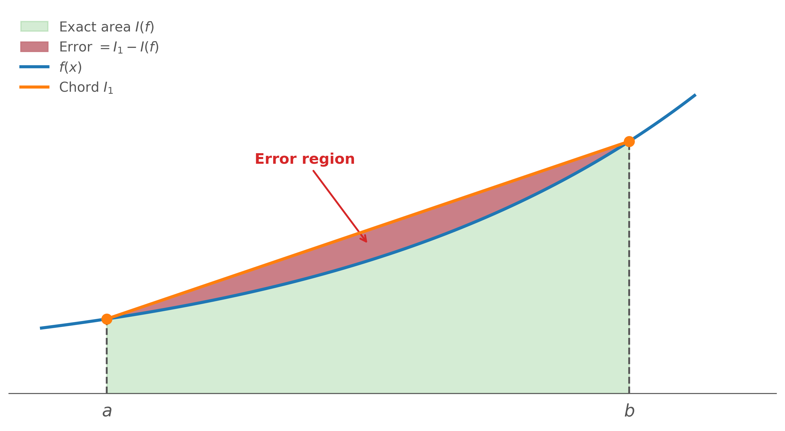
Concave-up f(x) with a trapezoidal chord lying above it; the blue region is the exact integral I(f) and the red region between the chord and f(x) is the overestimation error I_1 minus I(f).

For a convex function (f′′(x)>0f''(x) > 0 throughout [a,b][a,b]), the chord lies strictly above the curve, and the red region represents the entire overestimation I1−I(f)I_1 - I(f).


Effect of Higher-Degree Rules

RuleOrder nnLeading Error TermError vs. (b−a)(b-a)
Trapezoidal1M212(b−a)3\dfrac{M_2}{12}(b-a)^3O ⁣((b−a)3)O\!\left((b-a)^3\right)
Simpson’s2M490(b−a)5\dfrac{M_4}{90}(b-a)^5O ⁣((b−a)5)O\!\left((b-a)^5\right)

Two observations follow immediately:

  1. Higher-degree rules are more accurate on a fixed interval. Simpson’s Rule introduces an error proportional to (b−a)5(b-a)^5 rather than (b−a)3(b-a)^3. For a moderately sized interval this is a dramatic reduction.

  2. The Composite Trapezoidal Rule trades interval size for accuracy. Using mm sub-intervals each of width h=(b−a)/mh = (b-a)/m, the error per sub-interval is O(h3)O(h^3) and the total error is m×O(h3)=O(h2)m \times O(h^3) = O(h^2). Doubling mm halves hh and reduces the total error by a factor of approximately 4.